Speciální funkce definovaná integrálem
Si (x) (modrá) a Ci (x) (zelená) vynesené na stejném grafu.
v matematika , trigonometrické integrály plocha rodina z integrály zahrnující trigonometrické funkce .
Sinusový integrál Spiknutí Si (X ) pro 0 ≤ X ≤ 8 π .
Odlišný sinus integrální definice jsou
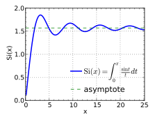
Si ( X ) = ∫ 0 X hřích t t d t { displaystyle operatorname {Si} (x) = int _ {0} ^ {x} { frac { sin t} {t}} , dt} si ( X ) = − ∫ X ∞ hřích t t d t . { displaystyle operatorname {si} (x) = - int _ {x} ^ { infty} { frac { sin t} {t}} , dt ~.} Všimněte si, že integrandhřích X X funkce sinc a také nula sférická Besselova funkce .Od té doby upřímně je dokonce celá funkce (holomorfní přes celou složitou rovinu), Si je celé, liché a integrál v jeho definici lze vzít sebou jakoukoli cestu připojení koncových bodů.
Podle definice, Si (X ) je primitivní z hřích X / X jehož hodnota je nula v X = 0si (X ) je to primitivní, jehož hodnota je nula v X = ∞Dirichletův integrál ,
Si ( X ) − si ( X ) = ∫ 0 ∞ hřích t t d t = π 2 nebo Si ( X ) = π 2 + si ( X ) . { displaystyle operatorname {Si} (x) - operatorname {si} (x) = int _ {0} ^ { infty} { frac { sin t} {t}} , dt = { frac { pi} {2}} quad { text {nebo}} quad operatorname {Si} (x) = { frac { pi} {2}} + operatorname {si} (x) ~ .} v zpracování signálu , oscilace sinusové integrální příčiny přestřelení a vyzváněcí artefakty při použití filtr sinc , a frekvenční doména vyzvánění, pokud používáte zkrácený filtr sinc jako dolní propust .
Související je Gibbsův fenomén : Pokud je sinusový integrál považován za konvoluce funkce sinc s funkce stepu heaviside , to odpovídá zkrácení Fourierova řada , což je příčinou Gibbsova jevu.
Kosinový integrál Spiknutí Ci (X ) pro 0 < X ≤ 8π .
Odlišný kosinus integrální definice jsou
Cin ( X ) = ∫ 0 X 1 − cos t t d t , { displaystyle operatorname {Cin} (x) = int _ {0} ^ {x} { frac {1- cos t} {t}} operatorname {d} t ~,} Ci ( X ) = − ∫ X ∞ cos t t d t = y + ln X − ∫ 0 X 1 − cos t t d t pro | Arg ( X ) | < π , { displaystyle operatorname {Ci} (x) = - int _ {x} ^ { infty} { frac { cos t} {t}} operatorname {d} t = gamma + ln x- int _ {0} ^ {x} { frac {1- cos t} {t}} operatorname {d} t qquad ~ { text {for}} ~ left | operatorname {Arg} ( x) vpravo | < pi ~,} kde y ≈ 0,57721566 ... je Euler – Mascheroniho konstanta . Některé texty používají ci namísto Ci .
Ci (X ) je primitivní funkcí cos X / X (který zmizí jako X → ∞ { displaystyle x to infty}
Ci ( X ) = y + ln X − Cin ( X ) . { displaystyle operatorname {Ci} (x) = gamma + ln x- operatorname {Cin} (x) ~.} Cin je dokonce , celá funkce . Z tohoto důvodu některé texty zacházejí Cin jako primární funkce a odvodit Ci ve smyslu Cin .
Hyperbolický sinusový integrál The hyperbolický sinus integrál je definován jako
Shi ( X ) = ∫ 0 X sinh ( t ) t d t . { displaystyle operatorname {Shi} (x) = int _ {0} ^ {x} { frac { sinh (t)} {t}} , dt.} Souvisí to s obyčejným sinusovým integrálem
Si ( i X ) = i Shi ( X ) . { displaystyle operatorname {Si} (ix) = i operatorname {Shi} (x).} Hyperbolický kosinový integrál The hyperbolický kosinus integrál je
Chi ( X ) = y + ln X + ∫ 0 X hovno t − 1 t d t pro | Arg ( X ) | < π , { displaystyle operatorname {Chi} (x) = gamma + ln x + int _ {0} ^ {x} { frac {; cosh t-1 ;} {t}} operatorname {d } t qquad ~ { text {for}} ~ left | operatorname {Arg} (x) right | < pi ~,} kde y { displaystyle gamma} Euler – Mascheroniho konstanta .
Má rozšíření série
Chi ( X ) = y + ln ( X ) + X 2 4 + X 4 96 + X 6 4320 + X 8 322560 + X 10 36288000 + Ó ( X 12 ) . { displaystyle operatorname {Chi} (x) = gamma + ln (x) + { frac {x ^ {2}} {4}} + { frac {x ^ {4}} {96}} + { frac {x ^ {6}} {4320}} + { frac {x ^ {8}} {322560}} + { frac {x ^ {10}} {36288000}} + O (x ^ {12}).} Pomocné funkce Trigonometrické integrály lze chápat ve smyslu tzv. „Pomocných funkcí“
F ( X ) ≡ ∫ 0 ∞ hřích ( t ) t + X d t = ∫ 0 ∞ E − X t t 2 + 1 d t = Ci ( X ) hřích ( X ) + [ π 2 − Si ( X ) ] cos ( X ) , a G ( X ) ≡ ∫ 0 ∞ cos ( t ) t + X d t = ∫ 0 ∞ t E − X t t 2 + 1 d t = − Ci ( X ) cos ( X ) + [ π 2 − Si ( X ) ] hřích ( X ) . { displaystyle { begin {array} {rcl} f (x) & equiv & int _ {0} ^ { infty} { frac { sin (t)} {t + x}} mathrm { d} t & = & int _ {0} ^ { infty} { frac {e ^ {- xt}} {t ^ {2} +1}} mathrm {d} t & = & quad operatorname { Ci} (x) sin (x) + left [{ frac { pi} {2}} - operatorname {Si} (x) right] cos (x) ~, qquad { text { a}} g (x) & equiv & int _ {0} ^ { infty} { frac { cos (t)} {t + x}} mathrm {d} t & = & int _ {0} ^ { infty} { frac {te ^ {- xt}} {t ^ {2} +1}} mathrm {d} t & = & - operatorname {Ci} (x) cos ( x) + left [{ frac { pi} {2}} - operatorname {Si} (x) right] sin (x) ~. end {pole}}} Pomocí těchto funkcí lze trigonometrické integrály znovu vyjádřit jako (srov. Abramowitz & Stegun, str. 232 )
π 2 − Si ( X ) = − si ( X ) = F ( X ) cos ( X ) + G ( X ) hřích ( X ) , a Ci ( X ) = F ( X ) hřích ( X ) − G ( X ) cos ( X ) . { displaystyle { begin {pole} {rcl} { frac { pi} {2}} - operatorname {Si} (x) = - operatorname {si} (x) & = & f (x) cos (x) + g (x) sin (x) ~, qquad { text {a}} operatorname {Ci} (x) & = & f (x) sin (x) -g (x) cos (x) ~. end {pole}}} Nielsenova spirála Nielsenova spirála.
The spirála tvořeno parametrickým grafem si, ci je známá jako Nielsenova spirála.
X ( t ) = A × ci ( t ) { displaystyle x (t) = a krát operatorname {ci} (t)} y ( t ) = A × si ( t ) { displaystyle y (t) = a krát operatorname {si} (t)} Spirála úzce souvisí s Fresnelovy integrály a Eulerova spirála . Nielsenova spirála má aplikace při zpracování vidění, stavbě silnic a tratí a dalších oblastech.[Citace je zapotřebí
Expanze Pro vyhodnocení trigonometrických integrálů lze použít různé expanze, v závislosti na rozsahu argumentu.
Asymptotická řada (pro velké argumenty) Si ( X ) ∼ π 2 − cos X X ( 1 − 2 ! X 2 + 4 ! X 4 − 6 ! X 6 ⋯ ) − hřích X X ( 1 X − 3 ! X 3 + 5 ! X 5 − 7 ! X 7 ⋯ ) { displaystyle operatorname {Si} (x) sim { frac { pi} {2}} - { frac { cos x} {x}} vlevo (1 - { frac {2!} { x ^ {2}}} + { frac {4!} {x ^ {4}}} - { frac {6!} {x ^ {6}}} cdots right) - { frac { sin x} {x}} left ({ frac {1} {x}} - { frac {3!} {x ^ {3}}} + { frac {5!} {x ^ {5} }} - { frac {7!} {x ^ {7}}} cdots right)} Ci ( X ) ∼ hřích X X ( 1 − 2 ! X 2 + 4 ! X 4 − 6 ! X 6 ⋯ ) − cos X X ( 1 X − 3 ! X 3 + 5 ! X 5 − 7 ! X 7 ⋯ ) . { displaystyle operatorname {Ci} (x) sim { frac { sin x} {x}} vlevo (1 - { frac {2!} {x ^ {2}}} + { frac { 4!} {X ^ {4}}} - { frac {6!} {X ^ {6}}} cdots right) - { frac { cos x} {x}} left ({ frac {1} {x}} - { frac {3!} {x ^ {3}}} + { frac {5!} {x ^ {5}}} - { frac {7!} {x ^ {7}}} cdots right) ~.} Tyto série jsou asymptotické a divergentní, i když je lze použít pro odhady a dokonce i pro přesné vyhodnocení na ℜ (X ) ≫ 1 .
Konvergentní série Si ( X ) = ∑ n = 0 ∞ ( − 1 ) n X 2 n + 1 ( 2 n + 1 ) ( 2 n + 1 ) ! = X − X 3 3 ! ⋅ 3 + X 5 5 ! ⋅ 5 − X 7 7 ! ⋅ 7 ± ⋯ { displaystyle operatorname {Si} (x) = součet _ {n = 0} ^ { infty} { frac {(-1) ^ {n} x ^ {2n + 1}} {(2n + 1 ) (2n + 1)!}} = X - { frac {x ^ {3}} {3! Cdot 3}} + { frac {x ^ {5}} {5! Cdot 5}} - { frac {x ^ {7}} {7! cdot 7}} pm cdots} Ci ( X ) = y + ln X + ∑ n = 1 ∞ ( − 1 ) n X 2 n 2 n ( 2 n ) ! = y + ln X − X 2 2 ! ⋅ 2 + X 4 4 ! ⋅ 4 ∓ ⋯ { displaystyle operatorname {Ci} (x) = gamma + ln x + sum _ {n = 1} ^ { infty} { frac {(-1) ^ {n} x ^ {2n}} { 2n (2n)!}} = Gamma + ln x - { frac {x ^ {2}} {2! Cdot 2}} + { frac {x ^ {4}} {4! Cdot 4 }} mp cdots} Tyto řady jsou konvergentní v každém komplexu X , i když pro |X , bude se série zpočátku pomalu sbíhat, což vyžaduje mnoho výrazů pro vysokou přesnost.
Odvození rozšíření série hřích X = X − X 3 3 ! + X 5 5 ! − X 7 7 ! + X 9 9 ! − X 11 11 ! + . . . { displaystyle sin , x = x - { frac {x ^ {3}} {3!}} + { frac {x ^ {5}} {5!}} - { frac {x ^ { 7}} {7!}} + { Frac {x ^ {9}} {9!}} - { frac {x ^ {11}} {11!}} + , ...}
hřích X X = 1 − X 2 3 ! + X 4 5 ! − X 6 7 ! + X 8 9 ! − X 10 11 ! + . . . { displaystyle { frac { sin , x} {x}} = 1 - { frac {x ^ {2}} {3!}} + { frac {x ^ {4}} {5!} } - { frac {x ^ {6}} {7!}} + { frac {x ^ {8}} {9!}} - { frac {x ^ {10}} {11!}} + , ...}
∴ ∫ hřích X X d X = X − X 3 3 ! ⋅ 3 + X 5 5 ! ⋅ 5 − X 7 7 ! ⋅ 7 + X 9 9 ! ⋅ 9 − X 11 11 ! ⋅ 11 + . . . { displaystyle proto int { frac { sin , x} {x}} dx = x - { frac {x ^ {3}} {3! cdot 3}} + { frac {x ^ {5}} {5! Cdot 5}} - { frac {x ^ {7}} {7! Cdot 7}} + { frac {x ^ {9}} {9! Cdot 9}} - { frac {x ^ {11}} {11! cdot 11}} + , ...}
Vztah s exponenciálním integrálem imaginárního argumentu Funkce
E 1 ( z ) = ∫ 1 ∞ exp ( − z t ) t d t pro ℜ ( z ) ≥ 0 { displaystyle operatorname {E} _ {1} (z) = int _ {1} ^ { infty} { frac { exp (-zt)} {t}} , dt qquad ~ { text {pro}} ~ Re (z) geq 0} se nazývá exponenciální integrál . Je to úzce spjato s Si a Ci ,
E 1 ( i X ) = i ( − π 2 + Si ( X ) ) − Ci ( X ) = i si ( X ) − ci ( X ) pro X > 0 . { displaystyle operatorname {E} _ {1} (ix) = i left (- { frac { pi} {2}} + operatorname {Si} (x) right) - operatorname {Ci} (x) = i operatorname {si} (x) - operatorname {ci} (x) qquad ~ { text {for}} ~ x> 0 ~.} Jelikož každá příslušná funkce je analytická, s výjimkou snížení záporných hodnot argumentu, oblast platnosti relace by měla být rozšířena na (Mimo tento rozsah jsou další termíny, které jsou celočíselnými faktory π
Případy imaginárního argumentu zobecněné integro-exponenciální funkce jsou
∫ 1 ∞ cos ( A X ) ln X X d X = − π 2 24 + y ( y 2 + ln A ) + ln 2 A 2 + ∑ n ≥ 1 ( − A 2 ) n ( 2 n ) ! ( 2 n ) 2 , { displaystyle int _ {1} ^ { infty} cos (sekera) { frac { ln x} {x}} , dx = - { frac { pi ^ {2}} {24} } + gamma left ({ frac { gamma} {2}} + ln a right) + { frac { ln ^ {2} a} {2}} + sum _ {n geq 1} { frac {(-a ^ {2}) ^ {n}} {(2n)! (2n) ^ {2}}} ~,} což je skutečná část
∫ 1 ∞ E i A X ln X X d X = − π 2 24 + y ( y 2 + ln A ) + ln 2 A 2 − π 2 i ( y + ln A ) + ∑ n ≥ 1 ( i A ) n n ! n 2 . { displaystyle int _ {1} ^ { infty} e ^ {iax} { frac { ln x} {x}} , operatorname {d} x = - { frac { pi ^ {2 }} {24}} + gamma left ({ frac { gamma} {2}} + ln a right) + { frac { ln ^ {2} a} {2}} - { frac { pi} {2}} i left ( gamma + ln a right) + sum _ {n geq 1} { frac {(ia) ^ {n}} {n! n ^ { 2}}} ~.} Podobně
∫ 1 ∞ E i A X ln X X 2 d X = 1 + i A [ − π 2 24 + y ( y 2 + ln A − 1 ) + ln 2 A 2 − ln A + 1 ] + π A 2 ( y + ln A − 1 ) + ∑ n ≥ 1 ( i A ) n + 1 ( n + 1 ) ! n 2 . { displaystyle int _ {1} ^ { infty} e ^ {iax} { frac { ln x} {x ^ {2}}} , operatorname {d} x = 1 + ia left [ - { frac {; pi ^ {2}} {24}} + gamma left ({ frac { gamma} {2}} + ln a-1 right) + { frac { ln ^ {2} a} {2}} - ln a + 1 doprava] + { frac { pi a} {2}} { Bigl (} gamma + ln a-1 { Bigr) } + sum _ {n geq 1} { frac {(ia) ^ {n + 1}} {(n + 1)! n ^ {2}}} ~.} Efektivní hodnocení Apostati Padé konvergentní Taylorovy řady poskytují efektivní způsob vyhodnocení funkcí pro malé argumenty. Následující vzorce uvedené v Rowe et al. (2015),[1] 10−16 pro 0 ≤ X ≤ 4 ,
Si ( X ) ≈ X ⋅ ( 1 − 4.54393409816329991 ⋅ 10 − 2 ⋅ X 2 + 1.15457225751016682 ⋅ 10 − 3 ⋅ X 4 − 1.41018536821330254 ⋅ 10 − 5 ⋅ X 6 + 9.43280809438713025 ⋅ 10 − 8 ⋅ X 8 − 3.53201978997168357 ⋅ 10 − 10 ⋅ X 10 + 7.08240282274875911 ⋅ 10 − 13 ⋅ X 12 − 6.05338212010422477 ⋅ 10 − 16 ⋅ X 14 1 + 1.01162145739225565 ⋅ 10 − 2 ⋅ X 2 + 4.99175116169755106 ⋅ 10 − 5 ⋅ X 4 + 1.55654986308745614 ⋅ 10 − 7 ⋅ X 6 + 3.28067571055789734 ⋅ 10 − 10 ⋅ X 8 + 4.5049097575386581 ⋅ 10 − 13 ⋅ X 10 + 3.21107051193712168 ⋅ 10 − 16 ⋅ X 12 ) Ci ( X ) ≈ y + ln ( X ) + X 2 ⋅ ( − 0.25 + 7.51851524438898291 ⋅ 10 − 3 ⋅ X 2 − 1.27528342240267686 ⋅ 10 − 4 ⋅ X 4 + 1.05297363846239184 ⋅ 10 − 6 ⋅ X 6 − 4.68889508144848019 ⋅ 10 − 9 ⋅ X 8 + 1.06480802891189243 ⋅ 10 − 11 ⋅ X 10 − 9.93728488857585407 ⋅ 10 − 15 ⋅ X 12 1 + 1.1592605689110735 ⋅ 10 − 2 ⋅ X 2 + 6.72126800814254432 ⋅ 10 − 5 ⋅ X 4 + 2.55533277086129636 ⋅ 10 − 7 ⋅ X 6 + 6.97071295760958946 ⋅ 10 − 10 ⋅ X 8 + 1.38536352772778619 ⋅ 10 − 12 ⋅ X 10 + 1.89106054713059759 ⋅ 10 − 15 ⋅ X 12 + 1.39759616731376855 ⋅ 10 − 18 ⋅ X 14 ) { displaystyle { begin {pole} {rcl} operatorname {Si} (x) & cca & x cdot left ({ frac { begin {pole} {l} 1-4,54393409816329991 cdot 10 ^ {- 2} cdot x ^ {2} +1,15457225751016682 cdot 10 ^ {- 3} cdot x ^ {4} -1,41018536821330254 cdot 10 ^ {- 5} cdot x ^ {6} ~~~ + 9,43280809438713025 cdot 10 ^ {- 8} cdot x ^ {8} -3,53201978997168357 cdot 10 ^ {- 10} cdot x ^ {10} +7,08240282274875911 cdot 10 ^ {- 13} cdot x ^ {12} ~~~ -6.05338212010422477 cdot 10 ^ {- 16} cdot x ^ {14} end {pole}} { begin {pole} {l} 1 + 1,01162145739225565 cdot 10 ^ {- 2} cdot x ^ {2} +4,99175116169755106 cdot 10 ^ {- 5} cdot x ^ {4} +1,55654986308745614 cdot 10 ^ {- 7} cdot x ^ {6} ~~~ + 3,28067571055789734 cdot 10 ^ { -10} cdot x ^ {8} +4,5049097575386581 cdot 10 ^ {- 13} cdot x ^ {10} +3,21107051193712168 cdot 10 ^ {- 16} cdot x ^ {12} end {pole}} } right) & ~ & operatorname {Ci} (x) & cca & gamma + ln (x) + && x ^ {2} cdot left ({ frac { begin {array} {l} -0,25 + 7,51851524438898291 cdot 10 ^ {- 3} cdot x ^ {2} -1,27528342240267686 cdot 10 ^ {- 4} cdot x ^ {4} +1,05297363846239184 cdot 10 ^ {- 6} cdot x ^ {6} ~~~ -4,68889 508144848019 cdot 10 ^ {- 9} cdot x ^ {8} +1.06480802891189243 cdot 10 ^ {- 11} cdot x ^ {10} -9,93728488857585407 cdot 10 ^ {- 15} cdot x ^ {12} end {array}} { begin {array} {l} 1 + 1,1592605689110735 cdot 10 ^ {- 2} cdot x ^ {2} +6,72126800814254432 cdot 10 ^ {- 5} cdot x ^ { 4} +2,55533277086129636 cdot 10 ^ {- 7} cdot x ^ {6} ~~~ + 6.97071295760958946 cdot 10 ^ {- 10} cdot x ^ {8} +1.38536352772778619 cdot 10 ^ {- 12 } cdot x ^ {10} +1,89106054713059759 cdot 10 ^ {- 15} cdot x ^ {12} ~~~ + 1,39759616731376855 cdot 10 ^ {- 18} cdot x ^ {14} konec {pole}}} doprava) konec {pole}}} Integrály lze vyhodnotit nepřímo pomocí pomocných funkcí F ( X ) { displaystyle f (x)} G ( X ) { displaystyle g (x)}
Si ( X ) = π 2 − F ( X ) cos ( X ) − G ( X ) hřích ( X ) { displaystyle operatorname {Si} (x) = { frac { pi} {2}} - f (x) cos (x) -g (x) sin (x)} Ci ( X ) = F ( X ) hřích ( X ) − G ( X ) cos ( X ) { displaystyle operatorname {Ci} (x) = f (x) sin (x) -g (x) cos (x)} nebo ekvivalentně F ( X ) ≡ [ π 2 − Si ( X ) ] cos ( X ) + Ci ( X ) hřích ( X ) { displaystyle f (x) equiv left [{ frac { pi} {2}} - operatorname {Si} (x) right] cos (x) + operatorname {Ci} (x) hřích (x)} G ( X ) ≡ [ π 2 − Si ( X ) ] hřích ( X ) − Ci ( X ) cos ( X ) { displaystyle g (x) equiv left [{ frac { pi} {2}} - operatorname {Si} (x) right] sin (x) - operatorname {Ci} (x) cos (x)}
X ≥ 4 { displaystyle x geq 4} Racionální funkce Padé níže uvedené přibližné F ( X ) { displaystyle f (x)} G ( X ) { displaystyle g (x)} −16 :[1]
F ( X ) ≈ 1 X ⋅ ( 1 + 7.44437068161936700618 ⋅ 10 2 ⋅ X − 2 + 1.96396372895146869801 ⋅ 10 5 ⋅ X − 4 + 2.37750310125431834034 ⋅ 10 7 ⋅ X − 6 + 1.43073403821274636888 ⋅ 10 9 ⋅ X − 8 + 4.33736238870432522765 ⋅ 10 10 ⋅ X − 10 + 6.40533830574022022911 ⋅ 10 11 ⋅ X − 12 + 4.20968180571076940208 ⋅ 10 12 ⋅ X − 14 + 1.00795182980368574617 ⋅ 10 13 ⋅ X − 16 + 4.94816688199951963482 ⋅ 10 12 ⋅ X − 18 − 4.94701168645415959931 ⋅ 10 11 ⋅ X − 20 1 + 7.46437068161927678031 ⋅ 10 2 ⋅ X − 2 + 1.97865247031583951450 ⋅ 10 5 ⋅ X − 4 + 2.41535670165126845144 ⋅ 10 7 ⋅ X − 6 + 1.47478952192985464958 ⋅ 10 9 ⋅ X − 8 + 4.58595115847765779830 ⋅ 10 10 ⋅ X − 10 + 7.08501308149515401563 ⋅ 10 11 ⋅ X − 12 + 5.06084464593475076774 ⋅ 10 12 ⋅ X − 14 + 1.43468549171581016479 ⋅ 10 13 ⋅ X − 16 + 1.11535493509914254097 ⋅ 10 13 ⋅ X − 18 ) G ( X ) ≈ 1 X 2 ⋅ ( 1 + 8.1359520115168615 ⋅ 10 2 ⋅ X − 2 + 2.35239181626478200 ⋅ 10 5 ⋅ X − 4 + 3.12557570795778731 ⋅ 10 7 ⋅ X − 6 + 2.06297595146763354 ⋅ 10 9 ⋅ X − 8 + 6.83052205423625007 ⋅ 10 10 ⋅ X − 10 + 1.09049528450362786 ⋅ 10 12 ⋅ X − 12 + 7.57664583257834349 ⋅ 10 12 ⋅ X − 14 + 1.81004487464664575 ⋅ 10 13 ⋅ X − 16 + 6.43291613143049485 ⋅ 10 12 ⋅ X − 18 − 1.36517137670871689 ⋅ 10 12 ⋅ X − 20 1 + 8.19595201151451564 ⋅ 10 2 ⋅ X − 2 + 2.40036752835578777 ⋅ 10 5 ⋅ X − 4 + 3.26026661647090822 ⋅ 10 7 ⋅ X − 6 + 2.23355543278099360 ⋅ 10 9 ⋅ X − 8 + 7.87465017341829930 ⋅ 10 10 ⋅ X − 10 + 1.39866710696414565 ⋅ 10 12 ⋅ X − 12 + 1.17164723371736605 ⋅ 10 13 ⋅ X − 14 + 4.01839087307656620 ⋅ 10 13 ⋅ X − 16 + 3.99653257887490811 ⋅ 10 13 ⋅ X − 18 ) { displaystyle { begin {pole} {rcl} f (x) & cca & { dfrac {1} {x}} cdot left ({ frac { begin {pole} {l} 1 + 7,444437068161936700618 cdot 10 ^ {2} cdot x ^ {- 2} +1,96396372895146869801 cdot 10 ^ {5} cdot x ^ {- 4} +2,37750310125431834034 cdot 10 ^ {7} cdot x ^ {- 6} ~~~ + 1.43073403821274636888 cdot 10 ^ {9} cdot x ^ {- 8} +4.33736238870432522765 cdot 10 ^ {10} cdot x ^ {- 10} +6,40533830574022022911 cdot 10 ^ {11} cdot x ^ {- 12} ~~~ + 4,20968180571076940208 cdot 10 ^ {12} cdot x ^ {- 14} +1,00795182980368574617 cdot 10 ^ {13} cdot x ^ {- 16} +4,94816688199951963482 cdot 10 ^ {12} cdot x ^ {- 18} ~~~ -4.94701168645415959931 cdot 10 ^ {11} cdot x ^ {- 20} end {pole}} { begin {pole} {l} 1+ 7,46437068161927678031 cdot 10 ^ {2} cdot x ^ {- 2} + 1,97865247031583951450 cdot 10 ^ {5} cdot x ^ {- 4} +2,41535670165126845144 cdot 10 ^ {7} cdot x ^ {- 6} ~~~ + 1.47478952192985464958 cdot 10 ^ {9} cdot x ^ {- 8} +4.58595115847765779830 cdot 10 ^ {10} cdot x ^ {- 10} +7.08501308149515401563 cdot 10 ^ {11} cdot x ^ {- 12} ~~~ + 5,06084464593475076774 cdot 10 ^ {12} cdot x ^ {- 14} +1,43468549171581016479 cdot 10 ^ {13} cdot x ^ {- 16} +1.11535493509914254097 cdot 10 ^ {13} cdot x ^ {- 18} end {array}}} right) && g (x) & cca & { dfrac {1} {x ^ {2}}} cdot left ({ frac { begin {array} {l} 1 + 8.1359520115168615 cdot 10 ^ {2} cdot x ^ {- 2} +2,35239181626478200 cdot 10 ^ {5} cdot x ^ {- 4} +3,1257570795778731 cdot 10 ^ {7} cdot x ^ {- 6} ~~~ + 2,06297595146763354 cdot 10 ^ {9} cdot x ^ {- 8} +6,83052205423625007 cdot 10 ^ {10} cdot x ^ {- 10} +1,09049528450362786 cdot 10 ^ {12} cdot x ^ {- 12} ~~~ + 7,57664583257834349 cdot 10 ^ {12} cdot x ^ {- 14} +1.81004487464664575 cdot 10 ^ {13} cdot x ^ {- 16} +6,43291613143049485 cdot 10 ^ {12} cdot x ^ {- 18} ~~~ -1.36517137670871689 cdot 10 ^ {12} cdot x ^ {- 20} end {array}} { begin {array} {l} 1 + 8,955 95201151451564 cdot 10 ^ {2} cdot x ^ { -2} +2,40036752835578777 cdot 10 ^ {5} cdot x ^ {- 4} +3,26026661647090822 cdot 10 ^ {7} cdot x ^ {- 6} ~~~ + 2,23355543278099360 cdot 10 ^ {9 } cdot x ^ {- 8} +7,87465017341829930 cdot 10 ^ {10} cdot x ^ {- 10} +1,39866710696414565 cdot 10 ^ {12} cdot x ^ {- 12} ~~~ + 1,17164723371736605 cdot 10 ^ {13} cdot x ^ {- 14} +4.01839087307 656620 cdot 10 ^ {13} cdot x ^ {- 16} +3,99653257887490811 cdot 10 ^ {13} cdot x ^ {- 18} end {pole}}} vpravo) konec {pole} }} Viz také Reference Další čtení Mathar, R.J. (2009). "Numerické vyhodnocení oscilačního integrálu nad exp (iπ X )·X 1/X mezi 1 a ∞ ". Dodatek B. arXiv :0912.3844 matematika ]. Press, W.H .; Teukolsky, S.A .; Vetterling, W.T .; Flannery, B.P. (2007). „Oddíl 6.8.2 - Kosinové a sinusové integrály“ . Numerické recepty: Umění vědecké práce na počítači (3. vyd.). New York: Cambridge University Press. ISBN 978-0-521-88068-8 Sloughter, Dan. "Sine Integral Taylor série proof" (PDF) . Diferenční rovnice k diferenciálním rovnicím . Temme, N.M. (2010), „Exponenciální, logaritmické, sinusové a kosinové integrály“ , v Olver, Frank W. J. ; Lozier, Daniel M .; Boisvert, Ronald F .; Clark, Charles W. (eds.), NIST Handbook of Mathematical Functions ISBN 978-0-521-19225-5 PAN 2723248 externí odkazy 


![{ displaystyle { begin {array} {rcl} f (x) & equiv & int _ {0} ^ { infty} { frac { sin (t)} {t + x}} mathrm { d} t & = & int _ {0} ^ { infty} { frac {e ^ {- xt}} {t ^ {2} +1}} mathrm {d} t & = & quad operatorname { Ci} (x) sin (x) + left [{ frac { pi} {2}} - operatorname {Si} (x) right] cos (x) ~, qquad { text { a}} g (x) & equiv & int _ {0} ^ { infty} { frac { cos (t)} {t + x}} mathrm {d} t & = & int _ {0} ^ { infty} { frac {te ^ {- xt}} {t ^ {2} +1}} mathrm {d} t & = & - operatorname {Ci} (x) cos ( x) + left [{ frac { pi} {2}} - operatorname {Si} (x) right] sin (x) ~. end {pole}}}](https://wikimedia.org/api/rest_v1/media/math/render/svg/0ba629ad1268d23aebd6a03f14f6720e91fc3183)


![{ displaystyle int _ {1} ^ { infty} e ^ {iax} { frac { ln x} {x ^ {2}}} , operatorname {d} x = 1 + ia left [ - { frac {; pi ^ {2}} {24}} + gamma left ({ frac { gamma} {2}} + ln a-1 right) + { frac { ln ^ {2} a} {2}} - ln a + 1 doprava] + { frac { pi a} {2}} { Bigl (} gamma + ln a-1 { Bigr) } + sum _ {n geq 1} { frac {(ia) ^ {n + 1}} {(n + 1)! n ^ {2}}} ~.}](https://wikimedia.org/api/rest_v1/media/math/render/svg/bb531475b072416d7add59348d55361c50ba523c)


![{ displaystyle f (x) equiv left [{ frac { pi} {2}} - operatorname {Si} (x) right] cos (x) + operatorname {Ci} (x) hřích (x)}](https://wikimedia.org/api/rest_v1/media/math/render/svg/2a843910ab6cb92c362e68ac401c28c1e7cda148)
![{ displaystyle g (x) equiv left [{ frac { pi} {2}} - operatorname {Si} (x) right] sin (x) - operatorname {Ci} (x) cos (x)}](https://wikimedia.org/api/rest_v1/media/math/render/svg/5f74128afc0519376e13432f0e9f5b0bf6627de7)

